import hmclab
from hmclab.Samplers import HMC
import numpy

Creating your own inverse problem

This notebook will show the steps required to implement (HMC) sampling of your own defined inverse problem.

To illustrate the process we will implement the Styblisnky-Tang function in arbitrary dimensions. The class will be built piece by piece, to indicate all required objects.

To implement any distribution / likelihood / target, we need to inherit from hmclab.Distributions._AbstractDistribution. By doing this, we can make the sampler understand that we passed a distribution, as well as providing checks on all required methods and attributes.

Note: We will now go through the process of illustrating what happens when you implement a distribution yourself, in steps. I’ll do this in a trial-and-error fashion, to show what happens if you omit required parts. For the shorter technical version, I refer to the documentation of the abstract class hmclab.Distributions._AbstractDistribution, which illustrates the required abstract methods and attributes.

Gathering all the ingredients

We can create a class that defines nothing (yet) and only inherits from the abstract base class the following way:

class my_inverse_problem_class(hmclab.Distributions._AbstractDistribution):
    pass

We now have a class of this distribution, e.g. a template on how to construct it. To actually use it, we need an instance. Instances of classes are created in the following way:

try:
    target = my_inverse_problem_class()
except Exception as e:
    print(e)

Can't instantiate abstract class my_inverse_problem_class with abstract methods generate, gradient, misfit

Oops, that didn’t work! If we try to decipher the Python error we can actually understand why: the class is missing ‘abstract’ functions. Abstract functions are functions that we have to implement ourselves. The abstract base class is asking for the following functions:

1. gradient : A function to compute the gradient of the misfit function.

2. misfit : A function to compute the misfit function.

The required input of misfit and gradient is a numpy vector of shape (dimensions, 1). The outputs are respectively a float and a numpy vector of shape (dimensions, 1). This can also be found when printing the documentation:

print(f"Function: {hmclab.Distributions._AbstractDistribution.gradient.__name__}")
print(hmclab.Distributions._AbstractDistribution.gradient.__doc__)

print(f"Function: {hmclab.Distributions._AbstractDistribution.misfit.__name__}")
print(hmclab.Distributions._AbstractDistribution.misfit.__doc__)

Function: gradient
Compute gradient of distribution.

        Parameters
        ----------
        coordinates : numpy.ndarray
            Numpy array shaped as (dimensions, 1) representing a column vector
            containing the coordinates :math:`\mathbf{m}`.

        Returns
        -------
        gradient : numpy.ndarray
            The distribution misfit gradient :math:`\nabla_\mathbf{m}\chi`.


        The distribution misfit gradient is related to the distribution probability
        density as:

        .. math::

            \nabla_\mathbf{m} \chi_\text{distribution} (\mathbf{m}) = -
            \nabla_\mathbf{m} \log p(\mathbf{m}).


        This method is called many times in an HMC appraisal. It is therefore
        beneficial to optimize the implementation.

Function: misfit
Compute misfit of distribution.

        Misfit computation (e.g. log likelihood) of the distribution. This method is
        present in all implemented derived classes, and should be present, with this
        exact signature, in all user-implemented derived classes.

        Parameters
        ----------
        coordinates : numpy.ndarray
            Numpy array shaped as (dimensions, 1) representing a column vector
            containing the coordinates :math:`\mathbf{m}`.

        Returns
        -------
        misfit : float
            The distribution misfit :math:`\chi`.


        The distribution misfit is related to the distribution probability density as:

        .. math::

            \chi_\text{distribution} (\mathbf{m}) \propto -\log p(\mathbf{m}).


        This method is called many times in an HMC appraisal. It is therefore
        beneficial to optimize the implementation.

        Note that the distribution need not be normalized, except when using mixtures of
        distributions. Therefore, distributions for which the normalization constant is
        intractable should not be used in mixtures. These distributions can be combined
        using Bayes' rule with other mixtures.

The API reference of these methods can be found at _AbstractDistribution.gradient and _AbstractDistribution.misfit.

An empty target model: Brownian Motion

To start, we can make a mock class, with zero misfit everywhere. This was the easiest implementation of a distribution that I could think of.

This essentially is a uniform unbouded distribution. Because it is an unnormalizable distribution, it is actually an improper prior. However, that doesn’t stop us from creating a Markov chain over it.

A class based on this could look like the following:

class my_inverse_problem_class(hmclab.Distributions._AbstractDistribution):
    def misfit(self, m):
        return 0

    def gradient(self, m):
        return numpy.zeros((dimensions, 1))

    def generate(self, m):
        raise NotImplementedError()

Creating an instance of this class should work now we have implemented all the required functions:

try:
    target = my_inverse_problem_class()
except Exception as e:
    print(e)

Can't instantiate abstract class my_inverse_problem_class with abstract attributes: dimensions

The error changed! No complaints about missing methods. We now have a complaint about a missing attribute; dimensions. It turns out, to do any sampling, we still have to define in what dimension model space we are operating. We can set this property in the constructor in the following way:

class my_inverse_problem_class(hmclab.Distributions._AbstractDistribution):
    def __init__(self):
        self.dimensions = 2

    def misfit(self, m):
        return 0

    def gradient(self, m):
        return numpy.zeros((self.dimensions, 1))

    def generate(self, m):
        raise NotImplementedError()

try:
    target = my_inverse_problem_class()
except Exception as e:
    print(e)

No errors!!

Now that we have an instance of a distribution, we can supply it to a sampler. Let’s give Hamiltonian Monte Carlo a try. The only thing we need other than the target is a mass matrix and a sampler instance. Creating these and starting the sampler:

HMC().sample(
    "bin_samples/tutorial_3_empty_distribution.h5",
    target,
    proposals=3000,
    overwrite_existing_file=True,
)

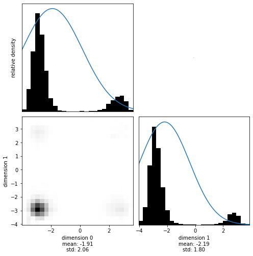
Visualizing the results shows how this empty class creates a Brownian motion. Brownian motion is simply a process that is independent of starting point and scale. Go ahead and change the time step of HMC or the amount of steps, histograms will always look similar (similarly random).

with hmclab.Samples("bin_samples/tutorial_3_empty_distribution.h5") as samples:
    hmclab.Visualization.marginal_grid(samples, [0, 1])

The Styblinsky-Tang Function

A more complete example would be to inplement some function as misfit and its derivative. One thing the following class implements is tempering, i.e. annealing. This changes a distribution to amplify or surpress local minima. This is a technique used in algorithms such as parallel tempering and simulated annealing. Tempering is implemented simply by dividing the misfit (and gradient) by the temperature.

You’re completely free to do the implementation of the gradient in any way you want (analytical derivatives, backpropagation, finite differences), however the accuracy to which the gradient is computed has direct influence on the performance of HMC. Getting it right (and fast) is typically essential to performant sampling with HMC.

The example demonstrated here is the n-dimensional tempered Styblinsky-Tang function. Its misfit is a sum of the same expression on every separate dimension, making the expression of the misfit and gradient rather simple. We don’t implement a generate function (as I wouldn’t know an effective way of generating samples), and we leave the dimensionality open to each instance.

class StyblinskiTang(hmclab.Distributions._AbstractDistribution):
    def __init__(self, dimensions=None, temperature=20.0):

        # Default to 2 dimensions if not specified
        if dimensions is None:
            self.dimensions = 2
        else:
            self.dimensions = dimensions

        # Default to temperature = 10 if not specified
        self.temperature = temperature

    def misfit(self, m):

        # Check the shape of the passed model
        assert m.shape == (self.dimensions, 1)

        return 0.5 * numpy.sum(m**4 - 16 * (m**2) + 5 * m) / self.temperature

    def gradient(self, m):

        assert m.shape == (self.dimensions, 1)

        return 0.5 * (4 * (m**3) - 32 * m + 5) / self.temperature

    def generate(self, m):
        raise NotImplementedError()

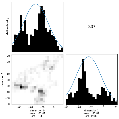
No errors is always good. Let’s try sampling this distribution at a temperature of 20.

target = StyblinskiTang(temperature=20)

HMC().sample(
    "bin_samples/tutorial_3_styblinski-tang.h5",
    target,
    proposals=20000,
    stepsize=1.0,
    overwrite_existing_file=True,
)

with hmclab.Samples("bin_samples/tutorial_3_styblinski-tang.h5") as samples:
    hmclab.Visualization.marginal_grid(samples, [0, 1], bins=25)

That looks great! Now you are ready to use the package on your interesting problems. Have fun!

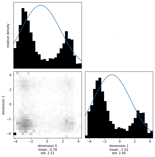
As a bonus, we can check what influence the tempering parameter has on the shape of the probability distribution. Reducing the temperature to 5 will ‘cool’ the distribution, sharpening it:

target = StyblinskiTang(temperature=5)

HMC().sample(
    "bin_samples/tutorial_3_styblinski-tang_cool.h5",
    target,
    proposals=20000,
    stepsize=0.5,
    overwrite_existing_file=True,
)

with hmclab.Samples("bin_samples/tutorial_3_styblinski-tang_cool.h5") as samples:
    hmclab.Visualization.marginal_grid(samples, [0, 1], bins=25)